Feature attribution in the Wavelet domain

Wavelets decompose signals into components that retain both spatial and frequency information, unlike Fourier transforms, which capture only frequency and discard spatial or temporal context. The choice of the wavelet determines what kind of structural components will be highlighted on the image. Its choice is therefore grounded in the application at hand.

A wavelet is a function $\psi \in \mathcal{H} = L^2(\mathbb{R}^n)$ that is normalized, centered at the origin, and has zero mean, i.e., $\int_{\mathbb{R}^n} \psi(x) \, dx = 0$. This function $\psi$ is called the mother wavelet, and it serves as the building block for constructing a family of wavelets via scaling and translation.

$$\psi_{\lambda,b}(x) = \frac{1}{\lambda^{n/2}} \, \psi\left(\frac{x - b}{\lambda} \right) \tag{1}$$

To analyze signals using wavelets, we often discretize the scale and translation parameters. A common and efficient choice is to use dyadic scales $\lambda = 2^j$ and translations on a dyadic grid $b = 2^j k$, where $j, k \in \mathbb{Z}$. This leads to the Discrete Wavelet Transform (DWT), based on the countable family:

$$\left\{ \psi_{j,k}(x) = 2^{j n/2}\, \psi\!\left(2^{j} x - k \right) \right\}_{j,k \in \mathbb{Z}} \tag{2}$$

The DWT represents a signal $g \in L^2(\mathbb{R}^n)$ by projecting it onto this family. The wavelet coefficients are obtained as inner products:

$$\mathcal{W}_{\mathrm{DWT}}(g)(j,k) = \langle g, \psi_{j,k} \rangle = \int_{\mathbb{R}^{n}} g(x)\,\overline{\psi_{j,k}(x)} \, dx \tag{3}$$

These coefficients measure the content of $g$ at scale $2^{-j}$ and location $2^{-j}k$. When $\psi$ satisfies certain admissibility and regularity conditions, the DWT becomes an invertible transform, and the signal can be exactly reconstructed:

$$\forall x\in\mathbb{R}^n,\quad g(x) = \sum_{\substack{j \in \mathbb{Z} \\ k \in \mathbb{Z}^n}} \langle g, \psi_{j,k} \rangle\psi_{j,k}(x), \tag{4}$$

where $\mathcal{W}_{\mathrm{DWT}}(g)(j,k)=\langle g, \psi_{j,k} \rangle$.

The figure below illustrates the process of decomposing an input image into its wavelet components.

Each dyadic wavelet coefficient $\mathcal{W}_{\mathrm{DWT}}(g)(j,k)$ quantifies the presence of features in the signal $g$ at a specific scale $2^{-j}$ and location $2^{-j}k$. Large coefficients indicate that the signal contains structures similar to the mother wavelet $\psi$ at that scale and position. In images, for example, these coefficients can highlight edges, textures, or other localized patterns, depending on the properties of $\psi$.

The multiscale and localized nature of the wavelet transform allows for the analysis of both fine and coarse features, making it especially powerful for signals with hierarchical or spatially varying content.

The selection of the mother wavelet $\psi$ depends on the application. Haar wavelets are well-suited for detecting sharp discontinuities, while smoother wavelets like Daubechies are better for representing gradual transitions.

In practice, the choice is guided by the characteristics of the data and the goals of the analysis. For image processing, wavelets that are localized in both space and frequency and have directional sensitivity are often preferred. The interpretability and effectiveness of the wavelet decomposition are directly linked to how well the chosen $\psi$ matches the underlying structures in the data.

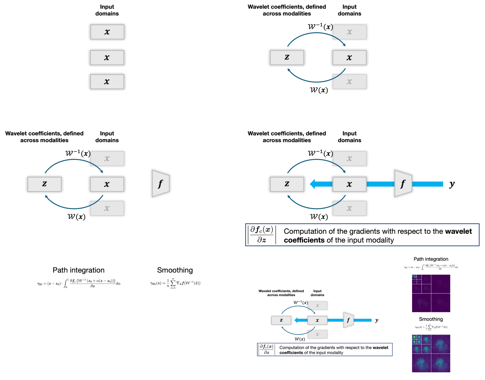
Let $\mathbf{f}$ be a classifier and $\mathbf{x}$ an input signal (e.g., an image, an audio, or a volume). The classifier maps the input to a class $c$ via $$ \mathbf{y}_c = \arg\max_{c \in \mathcal{C}} \mathbf{f}(\mathbf{x}) \equiv \mathbf{f}_c(\mathbf{x}), $$ with a slight abuse of notation. The original saliency map for class $c$ is defined as: $$ \gamma_{\text{Sa}}(\mathbf{x}) = \left| \nabla_{\mathbf{x}} \mathbf{f}_c(\mathbf{x}) \right|, $$ where $\mathbf{f}_c$ is assumed to be piecewise differentiable (Simonyan et al., 2014). This map highlights the components of the input $\mathbf{x}$ that most influence the classifier's decision, based on the gradient's magnitude.

Let $\mathbf{z} = \mathcal{W}(\mathbf{x})$ denote the discrete wavelet transform (DWT) of $\mathbf{x}$. Since $\mathcal{W}$ is invertible, we can define the saliency map in the wavelet domain as:

$$ \gamma_{\text{Sa}}(\mathbf{z}) = \left| \frac{\partial \mathbf{f}_c(\mathbf{x})}{\partial \mathbf{z}} \right| = \left| \frac{\partial \mathbf{f}_c(\mathbf{x})}{\partial \mathbf{x}} \cdot \frac{\partial \mathcal{W}^{-1}(\mathbf{z})}{\partial \mathbf{z}} \right|, \tag{5} $$

using the relation $\mathbf{x} = \mathcal{W}^{-1}(\mathbf{z})$ and the chain rule. The first term is the gradient of the classifier with respect to the input, and the second is the Jacobian of the inverse wavelet transform. This wavelet-domain saliency map tells us which coefficients — localized in both space and frequency — are most relevant for the prediction.

Smoothing

Since $\mathbf{f}_c$ is not necessarily continuously differentiable, the raw gradients can vary abruptly, especially at fine scales. To address this, we apply a smoothing strategy inspired by SmoothGrad (Smilkov et al., 2017), which averages gradients over a set of noisy inputs.

$$ \gamma_{\text{SG}}(\mathbf{z}) = \frac{1}{n} \sum_{i=1}^{n} \nabla_{\tilde{\mathbf{z}}} \mathbf{f}\left( \mathcal{W}^{-1}(\tilde{\mathbf{z}}) \right), \tag{6} $$

where $\tilde{\mathbf{z}} = \mathcal{W}(\mathbf{x} + \boldsymbol{\delta})$ and $\boldsymbol{\delta} \sim \mathcal{N}(0, \sigma^2 I)$. The number of samples $n$ and noise level $\sigma^2$ are tunable hyperparameters. This produces more stable and interpretable saliency maps in the wavelet domain.

Path Integration

An alternative to smoothing is to average gradients along a continuous path from a baseline input $\mathbf{x}_0$ (typically set to zero) to the actual input. This method, known as Integrated Gradients ( Sundararajan et al., 2017), satisfies desirable theoretical properties like sensitivity and implementation invariance.

Adapting this method to the wavelet domain, let $\mathbf{z} = \mathcal{W}(\mathbf{x})$ and $\mathbf{z}_0 = \mathcal{W}(\mathbf{x}_0)$, then we define:

$$ \gamma_{\text{IG}}(\mathbf{z}) = (\mathbf{z} - \mathbf{z}_0) \cdot \int_0^1 \frac{\partial \mathbf{f}_c\left( \mathcal{W}^{-1}(\mathbf{z}_0 + \alpha(\mathbf{z} - \mathbf{z}_0)) \right)}{\partial \mathbf{z}} \, d\alpha. \tag{7} $$

This formulation attributes importance to each wavelet coefficient by integrating its effect along a straight-line path in the wavelet domain.